Optimization in R

Finding the peak of parabola

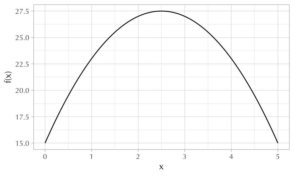
\[y = 15 + 10x - 2x^2\]

First we write this statement as an R function.

Code

parabola <- function(x) 15 + 10*x - 2*x^2

Then we can visualize it using curve() or ggplot2.

Code

library(ggplot2)
theme_set(theme_light(base_family = "Optima"))

g <- ggplot() + 
  geom_function(fun = parabola) +
  xlim(0, 5) +
  labs(x = "x", y = "f(x)")

g

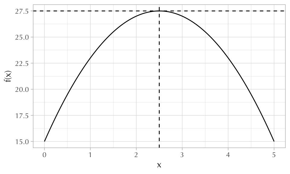
Then we call optimize(), which takes the function as its first argument, the interval as its second, and an optional argument indicating whether or not you are searching for the function’s maximum (minimize is the default).

Code

out <- optimize(parabola, interval = c(-100, 100), maximum = TRUE)
out

$maximum
[1] 2.5

$objective
[1] 27.5

Code

g + geom_vline(xintercept = out$maximum, linetype = "dashed") +
    geom_hline(yintercept = out$objective, linetype = "dashed")

There are many more ways of using optimization in R. For example, if you want to find the maximum of a function with many parameters you can use optim().

Code

opt <- optim(
  par = 99, ## initial values; use c(...) to do it with many parameters
  fn = parabola, 
  method = "BFGS",
  # this next line is critical: 
  # it tells R to maximize rather than minimize
  control = list(fnscale = -1)
)

opt

$par
[1] 2.5

$value
[1] 27.5

$counts
function gradient 
       6        3 

$convergence
[1] 0

$message
NULL

Logistic Regression

In statistics we usually try to find the maximum of likelihood functions in order to fit regression models.

For example¹, a simple logistic regression can be fit by doing the following:

Code

## The dataset
data("wells", package = "rstanarm")
str(wells)

'data.frame':   3020 obs. of  5 variables:
 $ switch : int  1 1 0 1 1 1 1 1 1 1 ...
 $ arsenic: num  2.36 0.71 2.07 1.15 1.1 3.9 2.97 3.24 3.28 2.52 ...
 $ dist   : num  16.8 47.3 21 21.5 40.9 ...
 $ assoc  : int  0 0 0 0 1 1 1 0 1 1 ...
 $ educ   : int  0 0 10 12 14 9 4 10 0 0 ...

Code

## The model
f <- formula(switch ~ dist + arsenic + dist:arsenic)

## The design matrix
X <- model.matrix(f, data = wells)
dim(X)

[1] 3020    4

Code

## The outcome variable
y <- wells$switch

## The log-likelihood function
log_likelihood <- function(beta, outcome, dmat) {
  
  linpred <- dmat %*% beta ## the linear predictor
  p <- plogis(linpred)     ## the link function
  
  sum(dbinom(outcome, size = 1, prob = p, log = TRUE))  ## the log-likelihood
}

## The maximum likelihood estimate (MLE)
opt <- optim(
  par = rep(0, ncol(X)), ## initial values are all 0's
  fn = log_likelihood, method = "BFGS",
  outcome = y, dmat = X,
  # this next line is critical: 
  # it tells R to maximize rather than minimize
  control = list(fnscale = -1)
)

names(opt$par) <- colnames(X)
opt$par

 (Intercept)         dist      arsenic dist:arsenic 
-0.147139626 -0.005811349  0.555574583 -0.001768792

We can compare this to the outcome given by R’s glm() function:

Code

fit <- glm(f, data = wells, family = binomial(link = "logit"))
coefficients(fit)

 (Intercept)         dist      arsenic dist:arsenic 
-0.147868069 -0.005772178  0.555976744 -0.001789060

Stan

Users of Stan should know that it can be used for optimization as well.

Code

library(cmdstanr)
mcmc_optim <- cmdstan_model("simple_parabola.stan")
mcmc_optim$print()

parameters {
  real<lower=0> x; // easily does constrained optimization
}

model {
  target += 15 + 10*x - 2*x^2;
}

Code

fit <- mcmc_optim$optimize()

Initial log joint probability = 17.7521 
    Iter      log prob        ||dx||      ||grad||       alpha      alpha0  # evals  Notes  
       4          27.5    0.00019008   2.86238e-06           1           1       12    
Optimization terminated normally:  
  Convergence detected: relative gradient magnitude is below tolerance 
Finished in  0.3 seconds.

Code

fit

 variable estimate
     lp__    27.50
     x        2.50

Footnotes

The data: «A survey of 3020 residents in a small area of Bangladesh suffering from arsenic contamination of groundwater. Respondents with elevated arsenic levels in their wells had been encouraged to switch their water source to a safe public or private well in the nearby area and the survey was conducted several years later to learn which of the affected residents had switched wells»↩︎